
Model-Based Tuning Methods for PID Controllers
- Home >
- articles >
- automation >
- pid controller design
Authors of this Article | ||
Jeffrey Arbogast Department of Chemical Engineering | Douglas J. Cooper, PhD Control Station, Inc. | Robert C. Rice, PhD Control Station, Inc. |
The manner in which a measured process variable responds over time to changes in the controller output signal is fundamental to the Design and tuning of a PID controller. The best way to learn about the dynamic behavior of a process is to perform experiments, commonly referred to as 'bump tests'. Critical to success is that the process data generated by the bump test be descriptive of actual process behavior. Discussed are the qualities required for 'good' dynamic data and methods for modeling the dynamic data for controller design. Parameters from the dynamic model are not only used in correlations to compute tuning values, but also provide insight into controller design parameters such as loop sample time and whether dead time presents a performance challenge. It is becoming increasingly common for dynamic studies to be performed with the controller in automatic (closed loop). For closed loop studies, the dynamic data is generated by bumping the set point. The method for using closed loop data is illustrated. Concepts in this work are illustrated using a level control simulation.
FORM OF THE CONTROLLER
The methods discussed here apply to the complete family of PID algorithms. Examples presented will explore the most popular controller of the PID family, the Proportional-Integral (PI) controller:
 [1]
[1]
In this controller, u(t) is the controller output and ![]() is the controller bias. The tuning parameters are controller gain,
is the controller bias. The tuning parameters are controller gain, ![]() , and reset time,
, and reset time, ![]() . Because
. Because ![]() is in the denominator, smaller values of reset time provide a larger weight to (increase the influence of) the integral term.
is in the denominator, smaller values of reset time provide a larger weight to (increase the influence of) the integral term.
CONTROLLER DESIGN PROCEDURE
Designing any controller from the family of PID algorithms entails the following steps:
Specifying the design level of operation,
Collecting dynamic process data as near as practical to this design level,
Fitting a first order plus dead time (FOPDT) model to the process data, and
Using the resulting model parameters in a correlation to obtain initial controller tuning values.
The form of the FOPDT dynamic model is:
 [2]
[2]
Where y(t) is the measured process variable and u(t) is the controller output signal. When Eq. 2 is fit to the test data, the all-important parameters that describe the dynamic behavior of the process result:
Steady State Process Gain,

Overall Process Time Constant,

Apparent Dead Time,

These three model parameters are important because they are used in correlations to compute initial tuning values for a variety of controllers [1]. The model parameters are also important because:
The sign of
 indicates the sense of the controller (+
 reverse acting; -
 direct acting)
The size of
 indicates the maximum desirable loop sample time (be sure sample time
  )
)The ratio
 indicates whether a Smith predictor would show benefit (useful if
  )
)The dynamic model itself can be employed within the architecture of feed forward, Smith predictor, decoupling and other model-based controller strategies.
DEFINING GOOD PROCESS TEST DATA
As discussed above, the collection and analysis of dynamic process data are critical steps in controller
Design and tuning. A 'good' set of data contains controller output to measured process variable data that
is descriptive of the dynamic character of the process. To obtain such a data set, the answer to all of
these questions about your data should be "yes" [1]. Ultimately, it is your responsibility to consider these steps to ensure success.
Was the process at steady state before data collection started?
Suppose a controller output change forces a dynamic response in a process, but the data file only shows
The tail end of the response without showing the actual controller output change that caused the
dynamics in the first place. Popular modeling tools will indeed fit a model to this data, but it will skew
the fit in an attempt to account for an unseen "invisible force." This model will not be descriptive of your actual process and hence of little value for control. To avoid this problem, it is important that data collection begin only after the process has settled out. The modeling tool can then properly account for all process variations when fitting the model.
Did the test dynamics clearly dominate the process noise?
When generating dynamic process data, it is important that the change in controller output cause a
Response in the process that clearly dominates the measurement noise. A rule of thumb is to define a
noise band of 3 standard deviations of the random error around the process variable during steady
operation. Then, when during data collection, the change in controller output should force the process
variable to move at least ten times this noise band (the signal to noise ratio should be greater than ten). If
you meet or exceed this requirement, the resulting process data set will be rich in the dynamic
information needed for controller design.
Were the disturbances quiet during the dynamic test?
It is essential that the test data contain process variable dynamics that have been clearly (and in the ideal
World exclusively) forced by changes in the controller output as discussed in step 2. Dynamics caused
by unmeasured disturbances can seriously degrade the accuracy of an analysis because the modeling tool
will model those behaviors as if they were the result of changes in the controller output signal. In fact, a
model fit can look perfect, yet a disturbance that occurred during data collection can cause the model fit
to be nonsense. If you suspect that a disturbance event has corrupted test data, it is conservative to rerun
the test.
Did the model fit appear to visually approximate the data plot?
It is important that the modeling tool display a plot that shows the model fit on top of the data. If the two
lines don't look similar, then the model fit is suspect. Of course, as discussed in step 3, if the data has
been corrupted by unmeasured disturbances, the model fit can look great yet the usefulness of the
analysis can be compromised.
NOISE BAND AND SIGNAL TO NOISE RATIO
When generating dynamic process data, it is important that the change in the controller output signal
Causes a response in the measured process variable that clearly dominates the measurement noise. One
way to quantify the amount of noise in the measured process variable is with a noise band.
As illustrated In Fig. 1, a noise band is based on the standard deviation of the random error in the
Measurement signal when the controller output is constant and the process is at steady state. Here the
noise band is defined as 3 standard deviations of the measurement noise around the steady state of the
measured process variable (99.7% of the signal trace is contained within the noise band). While other definitions of the noise band have been proposed, this definition is conservative when used for controller design.
When generating dynamic process data, the change in controller output should cause the measured process variable to move at least ten times the size of the noise band. Expressed concisely, the signal to noise ratio should be greater than ten. In Fig. 1, the noise band is 0.25°C. Hence, the controller output should be moved far and fast enough during a test to cause the measured exit temperature to move at least 2.5°C. This is a minimum specification. In practice it is conservative to exceed this value.
Noise Band of Heat Exchanger PV
Process: Heat Exchanger Controller: Manual Mode
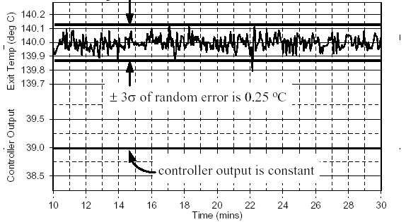
Figure 1 - Noise Band Encompasses 3 Standard Deviations Of The Measurement Noise
CONTROLLER TUNING FROM CORRELATIONS
The recommended tuning correlations for controllers from the PID family are the Internal Model Control
(IMC) relations [1]. These are an extension of the popular lambda tuning correlations and include the added
sophistication of directly accounting for dead time in the tuning computations.
The first step in using the IMC (lambda) tuning correlations is to compute, ![]() , the closed loop time
, the closed loop time
Constant. All time constants describe the speed or quickness of a response. The closed loop time constant
describes the desired speed or quickness of a controller in responding to a set point change. Hence, a small![]() (a short response time) implies an aggressive or quickly responding controller. The closed loop time constants are computed as:
(a short response time) implies an aggressive or quickly responding controller. The closed loop time constants are computed as:
Aggressive Tuning:
C τ Is the larger of 0.1 P τ Or 0.8 P θModerate Tuning:
C τ Is the larger of 1.0 P τ Or 8.0 P θConservative Tuning:
C τ Is the larger of 10 P τ or 80.0 P θWith °C computed, the PI correlations for IMC tuning are:
 [3]
[3]
Final tuning is verified on-line and may require tweaking. If the process is responding sluggishly to disturbances and changes in the set point, the controller gain is too small and/or the reset time is too large. Conversely, if the process is responding quickly and is oscillating to a degree that makes you uncomfortable, the controller gain is too large and/or the reset time is too small.
EXAMPLE: SET POINT TRACKING IN GRAVITY DRAINED TANKS
The gravity drained tanks process, shown In Fig. 2, is two non-interacting tanks stacked one above the
Other. Liquid drains freely through a hole in the bottom of each tank. As shown, the measured process
variable is liquid level in the lower tank. To maintain level, the controller manipulates the flow rate of liquid
entering the top tank. The disturbance variable is a secondary flow out of the lower tank from a positive
displacement pump. Thus, the disturbance flow is independent of liquid level.
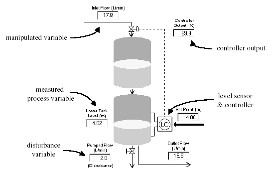
Figure 2 - Gravity Drained Tanks Process
The design level of operation for this study is a measured level in the lower tank of 2.4 m while the pumped flow disturbance is at its expected value of 2.0 L/min. The control objective is to track set point steps in the range of 2.0 to 2.8 m. The process is currently under P-Only control and operations personnel will not open the loop for controller design experiments. Hence, closed loop set point steps are used to generate dynamic process data.
As shown In Fig. 3, the P-Only controller being used has a ![]() = 40 %/m and a bias value of 55.2% (determined as the value of the controller output that, in open loop, causes the measured level in the lower tank to steady at the design value of 2.4 m when the pumped flow disturbance is at its expected value of 2.0 L/min). With data being saved to file, the dynamic testing experiment begins. Specifically, the set point is stepped up to 2.8 m, then down to 2.0 m, and finally back to the design level of 2.4 m (set point sequences of other sizes and durations would be equally reasonable).
= 40 %/m and a bias value of 55.2% (determined as the value of the controller output that, in open loop, causes the measured level in the lower tank to steady at the design value of 2.4 m when the pumped flow disturbance is at its expected value of 2.0 L/min). With data being saved to file, the dynamic testing experiment begins. Specifically, the set point is stepped up to 2.8 m, then down to 2.0 m, and finally back to the design level of 2.4 m (set point sequences of other sizes and durations would be equally reasonable).
P-Only Set Point Step Test
Process: Gravity Drained Tank Controller: PID ( P= RA, I= off, D= off )
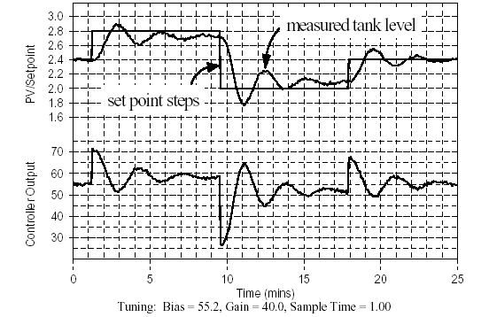
Figure 3 - Set point step tests on gravity drained tanks under P-Only control
Visual inspection of Fig. 3 confirms that the closed loop dynamic event is set point driven (as opposed to disturbance driven). Also, control action appears energetic enough such that the response of the measured process variable clearly dominates the noise.
FOPDT of Closed Loop Data
Model: First Order Plus Dead Time (FOPDT) File Name: closed.
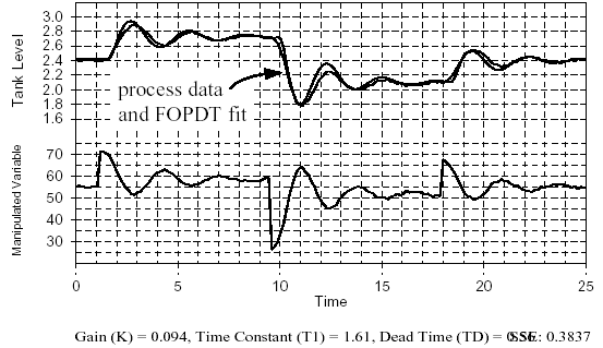
Figure 4 - FOPDT fit of closed loop dynamic data generated In Fig.8.5
The dynamic data of Fig. 3 is fit with a FOPDT model using Loop-Pro software by Control Station. A plot of the model and closed loop process data is shown in Fig. 4. The model appears to be reasonable and appropriate based on visual inspection, thus providing the design parameters:
Process Gain, KP = 0.094 m/%
Time Constant, τP = 1.6 min
Dead Time, θP = 0.56 min
We first compute the closed loop time constant. Here we choose aggressive tuning, which is computed as:
τC = larger of 0.1Ͽ�P or 0.8Ͽ�P = larger of 0.1(1.6) or 0.8(0.56) = 0.45 min.
Substituting this closed loop time constant and the above FOPDT model parameters into the IMC tuning correlations of Eq. 3 yields the following tuning values:

A reverse acting controller is required because KC is positive. Because the PI controller has integral action, the bias value is not entered but is automatically initialized by our instrumentation to the current value of the controller output at the moment the loop is closed.
PI Controller Design From P-Only Set Point Data
Process: Gravity Drained Tank Cont.: PID ( P= RA, I= ARW, D= off, F = off)
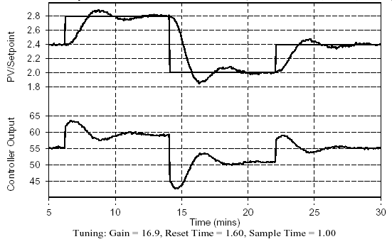
Figure 5 - Performance of PI controller in tracking set point steps
The performance of this controller in tracking set point changes is pictured In Fig. 5. Although good or best performance is decided based on the capabilities of the process, the goals of production, the impact on downstream units and the desires of management, Fig. 5 exhibits generally desirable performance. That is, the process responds quickly, shows modest overshoot, settles quickly, and displays no offset. Compare this to Fig. 3, that shows P-Only performance for the same control challenge.
INTERACTION OF PI TUNING PARAMETERS
One challenge of the PI controller is that there are two tuning parameters to adjust and difficulties can arise
Because these parameters interact with each other. Figure 6 shows a tuning map that illustrates how a
typical set point response might vary as the two tuning parameters are changed.
The center of Fig. 6 shows a set point step response that is labeled as the base case performance. It is
important to recognize that this base case plot will not be considered by some to be the "best" performance.
What is best must be determined by the operator or engineer for each implementation. Some require no
overshoot while others will tolerate some overshoot in exchange for a faster set point response. In any
event, the grid shows how a set point step response changes as the two tuning parameters are doubled and
halved from a base (here defined as desired) tuning.
PI Controller Tuning Map
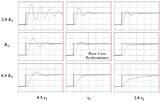
Figure 6 - How PI controller tuning parameters impact set point tracking performance
The plot in the upper left of the grid shows that when gain is doubled and reset time is halved, the controller produces large, slowly damping oscillations. Conversely, the plot in the lower right of the grid shows that when controller gain is halved and reset time is doubled, the response becomes sluggish. This chart is called a tuning map because, in general, if a controller is behaving poorly, you can match the performance you observe with the closest picture in Fig. 6 and obtain guidance as to the appropriate tuning adjustments required to move toward your desired performance.
CONCLUSIONS
Understanding the dynamic behavior of a process is essential to the proper design and tuning of a PID
Controller. The recommended design and tuning methodology is to:
Step, pulse or otherwise perturb the controller output near the design level of operation,
Record the controller output and measured process variable data as the process responds, and
Fit a first order plus dead time (FOPDT) dynamic model to this process data,
Use the dynamic model parameters in a correlation to compute P-Only, PI, PID and PID with Filter
Test your controller to ensure satisfactory performance.
LITERATURE CITED
1. Cooper, Douglas, "Practical Process Control Using Control Station", Published by Control Station,
Inc, Storrs, CT (2004).
For more information about model-based tuning techniques and technologies, please see our other resources below:
PID Tuning Blueprint, Calculator and Simulator Download
Right click, 'save target as' to download "Model-Based Tuning Methods for PID Controllers" (10 pages)
Right click, 'Save Target As' to download "Performance Monitoring Fundamentals" (17 pages)
Feel free to contact Control Station, Inc. Who donated this article to us.
Control Station, Inc. One Technology Drive Tolland, Connecticut 06084 877-LOOP-PRO (877-566-7776)
